August 16, 2021
![]() Pytorch is an open source deep learning framework. It provides a fast development to production deployment. It also built to make use of GPU’s for faster training.
Pytorch is an open source deep learning framework. It provides a fast development to production deployment. It also built to make use of GPU’s for faster training.
Tensors encode the inputs and outputs of a model and its parameters. They are a data structure that are similar to NumPy ndarrays. Because tensors can run on GPUs, they can run even faster than NumPy which is already a numbers optimizer for Python. So, the good news is that if you already know how to manipulate NumPy arrays, then tenors are same. You can even convert one to the other very easily.
August 17, 2021
Pytorch
I ran through the quick tutorial and when finished it seemed I needed to dust up on Neural Networks. That is where StatQuest came in handy. I’ve been getting small doses of statistics from Josh Starmer’s short vids on specifics of statistics. I am also reading a few books about stats so I’m getting a direct feed from different angles. The simplistic idea of Neural Networks is that they are fitting squiggly lines to the data instead of straight ones. On each synapse that connect the nodes, there are weights which multiply the x values and the biases that add or subtract from that value and the node of destination is training a certain model either Softmax, ReLU, or Sigmoid. After leaving the node, another set of calculations of weights and biases are applied. 
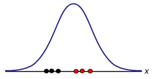
In a simple network, you have a starting node where the x-value passes through on a branching path to two different nodes on the next layer. This layer forms part of the hidden layer. On each connecting “synapse” between the nodes, different weights(multiplied) and biases (added/subtracted) are applied to the x value. These weights and biases come from back propagation that takes place in preprocessing. In each node of the new layer, a specified model is trained and then they are sent to a further layer. On the final layer (here, it’s the last node) another set of weights and biases are applied before summing the two paths and making one final adjustment. The results is a predicted value for y that is appropriate according to the calculations applied along the way.
Statquest
Now I am learning about FDRs (aka the Benjamini-Hochberg method). False Detection Rate intends to reduce the probability of false positives when sampling data and especially when taking a large number of samples from a distribution.
Let’s say you take 10,000 samples from a single distribution that has 10,000 measures. If your p-value threshold is at p<0.05 then you will have 5% False Positives among you samples. 5% of 10,000 is 500 which is not a small number. The distribution of p-values will be uniform. The red bar represents False Positives.
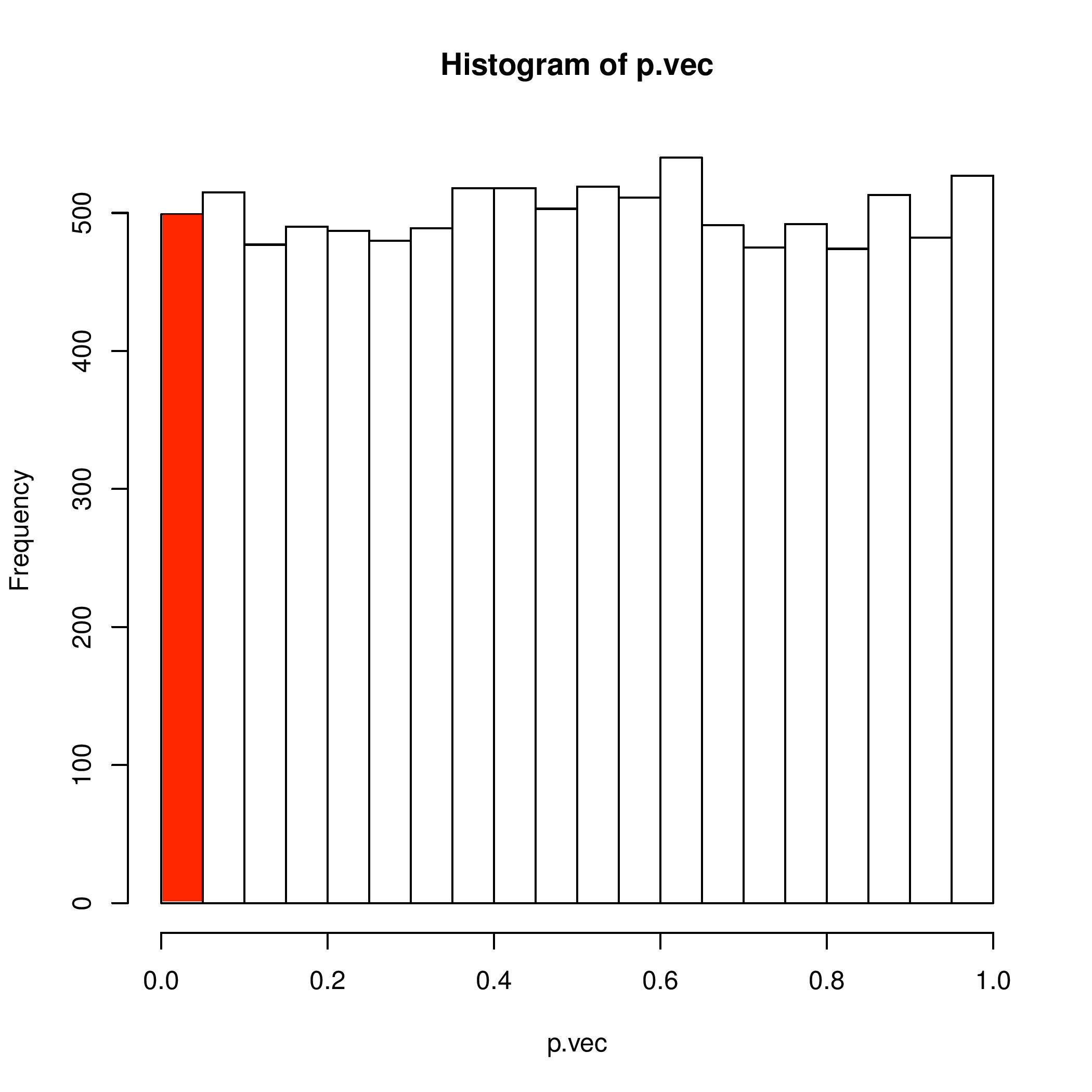
This means that each range of p-values will have the same probability of occurring. But this is when we are comparing two samples from the same distribution over 10,000 trails. The red bar is below the threshold of 0.05. Therefore, we know it is incorrect and the possibility of a False Positive is 5%. We can backwards engineer the process in order to see the naturally occurring frequency we are 100% confident that the samples come from the same distribution.
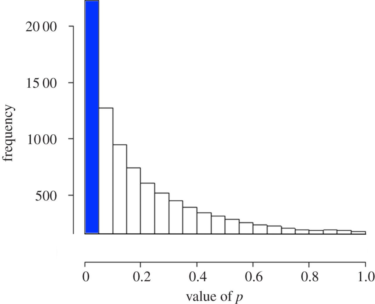
In contrast, if we take and compare two samples from two different distributions over many different trials, then the p-values will tend toward zero and skewed to the left. 95% of the results will have a p-value of less than 0.05. (Please ignore the figures of these plots, they only are for visual orientation of the principle.) The blue bar represents the True Positives.
Now, if we have undefined distributions and we don’t know if we are comparing two samples from the same distribution or from two different distributions then we have to estimate the uniformly distributed p-values (which would contain out False Positives) and separate those out of the p-values that are less than 0.05. We can be confident that what remains are the True Positives.
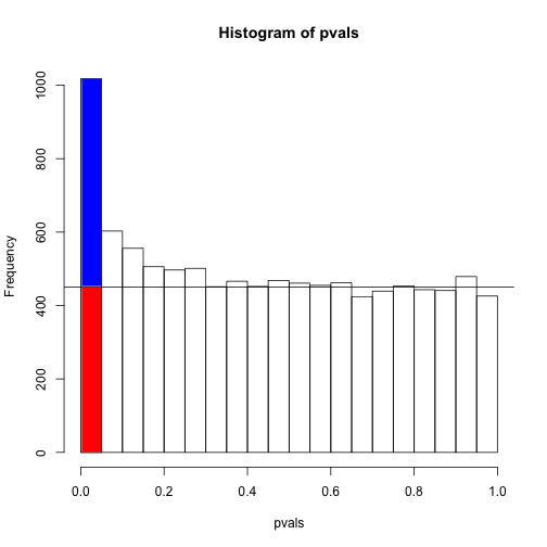
This is a visual demonstration of the principle of FDR and the Benjamini-Hochberg Method. The essential calculations will increase the p-values according to certain conditions that will cause the False Positives to have a value that is less statistically significant. For example, a “False Positive” 0.04 converts to “Fail to Reject Null” 0.06 after applying the method. But a true positive might convert from 0.01 to 0.045.